Exam ‘cheat sheets’ for EngSci 2nd year semester fall semester. These were made as part of my own studying for the exams. As 3/6 of my exams were cancelled due to the omicron covid variant, AER210, MAT292, and PHY293 are missing.

I do not guarantee content correctness – but if you find a mistake, please let me know!

CHE260

Note: the following only contains materials for the final exam, so it will only cover the heat-transfer portion of CHE260.

Variables

Below are some variables and what they generally mean in the context of CHE260

• \(k\): Thermal conductivity constant. Larger for good heat conductors, lower for ones that do so poorly
• \(h\): Convection heat transfer coefficient
• \(\alpha = \frac{k}{\rho c_p}\): Thermal diffusivity
• \(T_{film} = \frac{T_s + T_\infty}{2}\): Film temperature: estimated temperature at the convection layer

Heat Transfer Mechanisms

$$Q_{conduction} = -kA\frac{dT}{dx}$$ $$Q_{convection} = hA(T_s - T_\infty)$$ $$Q_{radiation} = \varepsilon\sigma A(T_s^4-T_{surr}^4)$$ Note: for radiation make sure to use Kelvin, not Celsius.

Steady Heat Transfer

We can apply the thermal resistance concept to build heat transfer resistance networks:

$$\dot{Q_{tot}} = \frac{T_2 - T_1}{R_{total}}$$

\(R_{total} \) is obtained through the various expressions for heat resistance for different shapes and methods. Draw out the resistance network and then solve for the total resistance which works in the same way as electrical resistance. Conduction resistances stacked perpendicular to the direction of heat flow are represented by parallel resistances.

For example, for two planes of glass,

$$R_T = R_{conv, 1} + R_{glass,1} + \\ R_{air} + R_{glass, 2} + R_{conv, 2}$$

Note the convection on either side.

The temperature at a point is is given using the heat transfer with resistance equation with a known total heat transfer and resistance between points \(a, b \), and temperature at one of the points.

$$Q_{a\rightarrow b} = \frac{T_a - T_b}{R_{a\rightarrow b}}$$

For spherical or cylindrical heat transfer there is a critical radius of insulation \(r_{cr} \) for which the heat transfer rate reaches a maximum, i.e. for \(r < r_{cr} \) the heat transfer rate is below maximum and will actually increase with added insulation until \(r = r_{cr} \), after which the heat transfer rate will go back down again.

• For a sphere: $$r_{cr} = \frac{2k_{ins}}{h}$$
• For a cylinder: $$r_{cr} = \frac{k_{ins}}{h}$$

Fins

For these problems just plug and chug.

$$a = \sqrt{\frac{hP}{kA_c}}$$

1. Infinitely long fin $$\frac{T(x) - T_\infty}{T_b - T_\infty} = exp(-ax)$$ $$\dot{Q} = \sqrt{kPkA_c}exp(-ax)$$

2. Adiabatic tip/insulated tip fin

$$\frac{T(x) - T_\infty}{T_b - T_\infty} = \frac{\cosh{a(L-x)}}{\cosh{aL}}$$ $$\dot{Q} = \sqrt{kPkA_c}(T_b - T_\infty)\tanh{aL}$$

where \(P \) is the perimeter of the fin and \(A_c \) is the cross-sectional area. \(h \) is the convection heat transfer coefficient of the surrounding fluid, and \(k \) the thermal conductivity constant for the fin material

Misc:

1. Fins exposed to convection at tips can be modelled as an adiabatic tip fin with a corrected length

$$L_c = L + \frac{A_c}{p}$$

2. Fin efficiency is the ratio of actual heat transfer (non-uniform temperature) to maximum heat transfer (uniform temperature)

$$\eta = \frac{\dot{Q_{tot}}}{\dot{Q_{tot\space max}}}$$

3. Fin effectiveness is the ratio of heat transfer due to fins to heat transfer if the fins were not present. \(A_b \) denotes the area of the fin bases, not that of the whole surface the fins are attached to.

$$\varepsilon = \frac{\dot{Q_{fin}}}{\dot{Q_{no\space fin}}} = \frac{\dot{Q_{fin}}}{hA_b(T_b-T\infty)}$$

4. Fin effectiveness and efficiency are related by

$$\varepsilon = \frac{A_{fin}}{A_{base}}\cdot\eta$$

Transient Heat Transfer

TLDR; modelling heat transfer as a function of time as well. If possible, apply lumped system assumption which assumes that the whole system has uniform temperature.

• Characteristic Length: \(L_c = \frac{V}{A_{surface}}\)
• Biot number: \(Bi = \frac{hL_c}{k}\)

Note: When we look up \(\lambda_1\) and \(A_1\) from tables make sure to use the same formula for Biot’s number as used by the reference source. The textbook uses \(Bi = \frac{hr_o}{k}\) for cylinders and spheres.

Lumped system approximation is valid for $$Bi \leq 0.1$$

We then can get the following by solving the heat equation

$$b = \frac{hA_s}{\rho c_p V} = \frac{h}{\rho c_p L_c}, [b] = s^{-1}$$

$$\frac{T(t) - T_\infty}{T_i - T_\infty} = e^{-bt}$$

Most questions will then get you to plug in the boundary conditions \(T_i, T(t), T_\infty\) and then have you solve for \(t\) or some combination thereof.

Procedure:

1. Determine \(L_c\)
2. Determine \(Bi\) and check if lumped system is valid
3. Plug into heat equation and solve for unknown

if \(Bi > 0.1\), then you will have to do some more work.

1. Assume \(\tau>0.2\) so one-term approximation is valid
2. Given \(Bi\), look up in reference table to find \(\lambda_1\) and \(A_1\)
3. Plug into the right expression for dimensionless temperature \(\theta = e^{-Bi*\tau}\). Below is the one-term expression for a plane wall. They all generally have a similar form.

$$\frac{T(x, t) - T_\infty}{T_i - T_\infty} = A_1e^{-\lambda_1^2\tau}\cos{\frac{\lambda_1 x}{L}}$$ and note that in this expression time is w.r.t. dimensionless time \(\tau\) – so to convert back to dimensioned time we apply $$\tau = \frac{\alpha t}{L^2}$$ to recover \(t\).

Note that at the center of a plane wall/cylinder/sphere/etc the above expression can be simplified to $$\frac{T(0, t) - T_\infty}{T_i - T_\infty} = A_1e^{-\lambda_1^2\tau}$$

For some questions (for example a plane wall cooled on both sides) we can express \(T(x,t)\) w.r.t \(T(0, t)\), i.e. \(T(x, t) = T(0, t)\cos{\lambda_1 x/L}\)

For heat transfer we express it as a % of the maximum heat transfer.

Given

$$Q_{max} = mc_p(T_\infty - T_i)$$

which denotes heat transfer as \(t\rightarrow\infty\)

we derive a ratio \(\frac{Q(t)}{Q_{max}}\) for different geometries, which should be given. \(Q(t)\) is the sum of internal energy changes throughout the entire geometry which can be expressed as a volume integral.

Semi-Infinite Solids

Used to model temperature change in part of body due to thermal conditions on a single surface TLDR; use this for questions where they don’t give you dimensions

$$\eta = \frac{x}{\sqrt{4\alpha t}}$$

For constant \(T_s\) we obtain

$$\frac{T(x,t)-T_i}{T_s-T_i} = erfc(\eta)$$

and

$$\dot{q}_s(t) = \frac{k(T_s-T_i)}{\sqrt{\pi\alpha t}}$$

where

$$erfc(\eta) = 1- \frac{2}{\sqrt{\pi}}\int^\eta_0 e^{-u^2}du$$

Generally we will be looking up \(\eta, erfc(\eta)\) in a table.

Forced Convection Heat Transfer

TLDR: What if we forced fluids instead of letting the convection happen naturally?

We know that

$$Q_{conv} = hA(T_s - T_\infty)$$

But how do we get \(h\) for forced convection? Either look it up from a table, get it experimentally, or do some math.

$$h=\frac{-k_{fluid}(\frac{\delta T}{\delta y}\vert_{y=0})}{T_s-T_\infty}$$ Note that the temperature distribution for a moving fluid isn’t constant. We can usually use an average one $$h=\frac{1}{A_s}\int_{A_s}h_{local}dA_s$$

Note: surface integral for the 2D case, and the over length \(L\) for the 1D.

In cases where the laminar flow region cannot be entirely disregarded, we must integrate over the parts separately

$$h = \frac{1}{L}(\int_0^{x_a} h_{x, laminar}dx + \\ \int_{x_a}^L h_{x, turbulent}dx)$$

Recall from AER210 the that fluid exerts a drag force \(\tau\) on the walls

$$\tau = \mu \frac{\delta\mu}{\delta y} \vert_{y=0}$$

Or,

$$\tau = c_f \frac{\rho v_o^2}{2}$$

where \(c_f\) is a friction coefficient which depends on geometry.

Forced convection is described with help from a few numbers

1. Reynold’s number \(Re\)

$$Re = \frac{\rho V_\infty D}{\mu} = \frac{V_\infty x}{\nu}$$ Note: \(\nu\) is kinematic viscosity \(\nu = \frac{\mu}{\rho}\)

Large \(Re\) tends towards turbulent flow, small tends towards laminar flow. Generally if \(Re<5*10^5\) the flow is laminar and it is turbulent otherwise.

2. Prachett’s number \(Pr\)

The ratio of molecular diffusivity of momentum over the molecular diffusivity of heat

$$Pr = \frac{v}{\alpha} = \frac{\mu c_p}{k}$$

3. Nusselt’s Number \(Nu\)

The dimensionless heat transfer coefficient which is the ratio of the convective heat transfer rate to the conductive heat transfer rate.

$$Nu = \frac{hL_c}{k}$$

We can then apply Buckingham \(\pi\) to represent \(Nu\) w.r.t. \(Re\) and \(Pr\).

$$Nu_x = \frac{h_xx}{k} = cRe_x^nPr^m$$

Note that here \(Nu\) is local to point \(x\)

And the coefficients \(c, m, n\) can either be solved for with experimental data or will be given. For example, for laminar flow over a flat plate:

$$Nu = \frac{hL}{k} = 0.664Re_L^{0.5}Pr^{(1/3)}, \\ Re_L < 5*10^5, Pr > 0.6$$

… and for turbulent flow: $$Nu = \frac{hL}{k} = 0.037Re_L^{0.8}Pr^{(1/3)}, \\ 5*10^5 \leq Re_L \leq 10^7, 0.6 \leq Pr \leq 60 $$

For isothermal surfaces with an unheated starting section of length \(\xi\) the local Nusselt’s number is given by

laminar :

$$Nu_x = \frac{hL}{k} = \frac{0.332Re_x^{0.5}Pr^{1/3}}{[1-(\xi/x)^{3/4}]^{1/3}}$$

turbulent :

$$Nu_x = \frac{hL}{k} = \frac{0.0296Re_x^{0.8}Pr^{1/3}}{[1-(\xi/x)^{910}]^{1/9}}$$

What is important to note here is that these equations are valid for an isothermal flat plate with an unheated starting section of length \(\xi=0\) as well. The equations would be the same as the two above except the denominator is 1. The previous equations (e.g. \(c=0.664\)) are valid for a flat plate heated at the leading edge.

Other:

• No-slip condition applies at walls, so right by the wall heat transfer is conductive. \(\dot{q} = \dot{q_{cond}}\)

Radiation Heat Transfer

For this section everything is just plug and chug and being careful with view factors. Most problems involve an energy balance \(\dot{q_{in}} = \dot{q_{out}} \)

1. Stefan-Boltzmann Law: $$E_b(T) = \sigma T^4$$

2. Wein’s displacement law: finding the wavelength that gives the maximum power for a specified surface temperature $$(\lambda T)_{max power} = 2897.8 \mu \cdot K$$

3. Reciprocity rule:

$$A_iF_{i\rightarrow j} = A_jF_{j\rightarrow i}$$

Where \(F_{i\rightarrow j} \) is the ‘view factor’, i.e. the percent of radiation leaving surface \(i \) that strikes surface \(j \) directly.

• \(\alpha = \frac{G_{absorbed}}{G} \): Absorptivity
• \(\rho = \frac{G_{reflected}}{G} \): Reflectivity
• \(\tau = \frac{G_{transmitted}}{G}\): Transmissivity

These variables also have the property

$$\alpha + \rho + \tau = 1$$

Note: for opaque surfaces \(\tau = 0 \)

4. Summation property: the set of view factors that describe radiation beginning at surface \(i \) and ending at all surfaces \(j \) that it touches has a sum of \(1 \).

$$\sum^N_{j=1}F_{ij} = 1$$

5. Putting all together When are looking at black body radiation only: $$\dot{Q_{1\rightarrow 2}} = A_1 F_{1\rightarrow 2} \sigma (T_1^4 - T_2^4)$$

Note: $$\dot{Q_{1\rightarrow 2}} = A_1\dot{q_{1\rightarrow 2}}$$

6. Heat transfer between surfaces

$$\dot{q_{12}} = \frac{\sigma(T_1^4-T_2^4)}{ \frac{1-\varepsilon_1}{A_1\varepsilon_1} + \frac{1}{A_1F_{12}} + \frac{1-\varepsilon_2}{A_2\varepsilon_2}}$$ Where the middle term in the denominator denotes the “resistivity” due to space and the other terms due to radiation.

So we can build resistance networks by adding up the resistances of each element here as well!

7. Kirchhoff’s law: Total emissivity of a surface is equal to the absorptivity for radiation coming from a black body at the same temperature

$$\varepsilon_\lambda(T) = \alpha_\lambda(T)$$

8. Radiosity: The radiation emitted + the radiation reflected by surface \(i \)

$$J_i = \varepsilon_i E_{bi} + (1-\varepsilon)G_i$$

Note that we know that for an opaque surface (\(\tau=0\)), \(\varepsilon + \rho = 1 \)

Other

• Radiation heat transfer coefficient \(h_{rad} \) provides radiative heat transfer as \(\dot{q} = h_{rad}(T_1-T_2)\)

ECE253: Digital and Computer Systems

Note: Hugo Chroma for armasm seems to be a little different from ARMv7 used. So the following code blocks will be highlighted with nasm syntax. Comments will be denoted with ‘;’ but should be ‘//’ in ARMv7.

Logic and Circuits

Karnaugh Maps

• Group w.r.t powers of 2.
• For 7-seg-display draw a K-map for each segment
• Minterm: Product term that evals to 1
• Maxterm: Sum term that evals to 0 Note that for minterms you don’t need to NOT it but for maxterms you do.
• Canonical POS: Maxterms that cover all 0s
• Canonical SOP: Minterms that cover all 1s
• Prime implicant: The largest group that can be covered by a single implicant
• Essential Prime Implicants: An implicant that covers a term that is not covered by any other implicant
• Find set comprised of most essential prime implicants – lowest cost cover

Other:

• Two’s complement: Flip bits and add 1. Leading 1 denotes negative number, leading 0 denotes positive number. E.x. 6 = 000100, -6 = 111001 + 1 = 111010.
• Finite State Machines
  • Draw out state table: |state|next w=0, w=1|output
  • Assign encodings to states e.g. A=1, B=2 .. or use one-hot
  • Reduce with K-maps; take columns on tables for K-map entries
  • Use a case statement or series of flip-flops to implement the FSM

Circuits to know

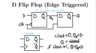D flip flop 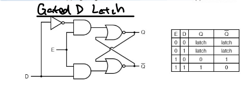Gated latch

Commonly used to storage a single bit of data. Can be chained together to store multiple bits of data, commonly as a shift register.

Verilog

Source: Operators

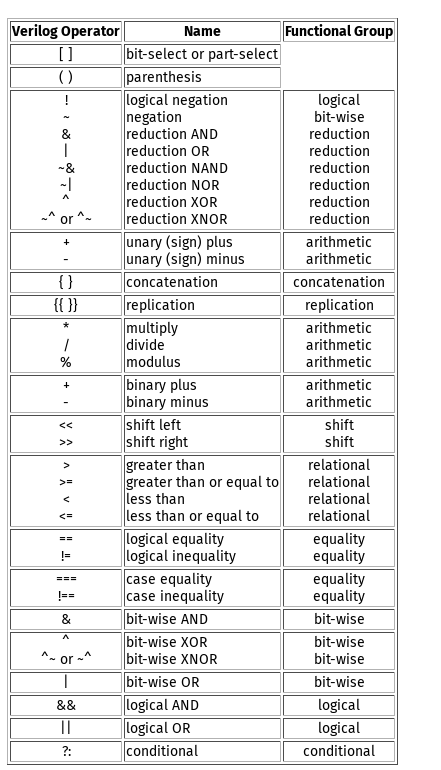
• Blocking vs Non-blocking

= is non-blocking, <= is blocking. For non-blocking = we treat the logic as combinatorial, and for blocking <= we treat the logic as sequential. So all the = steps can take one cycle (completed in parallel) while the <= steps can take multiple cycles (completed in sequence). With sequential logic, “step through” the behaviour of the circuit first and then it should be pretty clear how to build it.

• Latches: checks the value as long as clock is high
• Flip flops: check only on clock edge
• Active high: reset when 1
• Active low: reset when 0
• Synchronous: reset on the next clock edge that the flip flop is supposed to resond to
• Asynchronous: reset on the next clock edge at anytime
• Cost heuristic: # gates + # inputs where inputs is the # of inputs to gate. i.e. cost of a AND gate is 1 + 2 = 3 since it is 1 gate and 2 inputs

ARM Assembly

For De1-SOC

• Registers are 32 bit/4 bytes
• Each instruction is 32 bits/4bytes long
• Tricks:
• Can extract the lowest bits out of a register by ANDing it with a ones mask
• Left shift by n bits is equivalent to multiply by 2^n
• Right shift by n bits is equivalent to divide by 2^n
• Registers: R0-R12: General Purpose R13: Stack Pointer R14: Link Register R15: Program Counter R16: Status Register

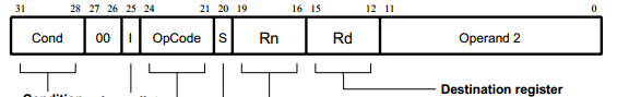
Opcode format:

We can load the top and bottom halves of registers into another like this:

1
2
3
4
5

; load the top half of R1 into R0
; and the bottom half of R3 into R0
MOV R0, R1
LSL R0, #16
ORR R0, R3

Instructions

Note that in the following I use O\d to denote an [O]perand which can be a register, a constant, or whatever else also works.

• MOV DEST, SRC
• LDR TARGET, [SOURCE, #offsetpos1], #offsetpos2. If using offsetpos1, SOURCE is pre-indexed, offsetpos2 post-index. When using with memory location or numeric literal, prepend =, i.e. LDR R0, =LIST or LDR R1, =0x0000000b
• LDR{OPT}, STR{OPT}, opt can be B: byte, H: halfword – if we only want to use part of it.
• STR DEST, [TARGET]
• CMP O1, O2: Compare O1 and O2 by computing O2 - O1 and then updating NZCV flags in the CPSR
• ADD O1, O2, O3: Add O2 to O3 and store the result in O1
• SUB O1, O2, O3: Subtracts O3 from O2 and store the result in O1
• ASR (Arithmetic Shift Right): Shift to the right, shifted in bits depend on leading sign bit
• LSL (Logical Shift Left): Shift to the left, shifted in bits are 0
• LSR (Logical Shift Right): Shift to the right, shifted in bits are 0
• MUL, O1, O2, O1: Multiply O1 by O2 and store the result in O1
• ORR, AND: Bitwise OR, AND

Note: MOV directly puts it into the destination register, LDR loads the value from the memory location into the destination register, STR stores the value from the source register into the memory location. When LDR is used with a literal it first loads the literal into memory and then loads the value from the memory location into the destination register.

• Conditional Execution Do CMP, then apply INSTR{COND} or do a branch Conditions: EQ, NE, GT, LT, GE, LE, S, -E denotes “or equal to”. S for add, subs updates N, Z, C, V flags

1
2

CMP R0, #3
ADDLT R0, R0, #1 ; adds 1 to R0 if R0 < 3

Using PC, LR

At instruction i, PC stores the address of the next instruction at i+1. The current instruction can be obtained via a negative offset ,#-4 LR by convention stores what we want to return to after a subroutine.

So, assuming that the first instruction of the following code chunk is stored at 0x0,

1
2
3
4
5
6

LDR R0, =0x2000 ; 0x00000000, PC: 0x00000004
MOV R2, #4    ; 0x00000004, PC: 0x00000008
BL ROUTINE ; 0x00000008, PC: 0x0000000C, LR 0x0000000C
MOV R2, #5 ; 0x0000000C, PC: 0x00000010
ROUTINE:
  PUSH {LR} ; 0x00000010, LR=0x0000000C

Subroutines

• Parameters are passed via R0-R3, which subroutines are free to modify and return with
• Subroutine should not modify the remaining registers; if so they should PUSH/POP to the stack before and after use
• Exit subroutine with MOV PC, LR
• BL is a branch and link instruction, which sets LR to the next instruction and sets PC to the label address

Stacks

• Must first initialize stack pointer, LDR SP, 0x20000

• Pushing to the stack pointer puts the value on top of the stack and decreases the stack pointer

• For many subroutines needing more than the default registers we want to push and pop the registers before and after we’re done.

• PUSH {Rs}: Pushs registers onto stack. Registers must be in ascending order and the largest one gets pushed in first. Has effect of decreasing the stack pointer.

• POP {Rs}: Pops data off the stack. Does not care what register the stack data comes from; i.e. PUSH {R5} POP {R6} would put R6 into R5. Can be used in recursion to put LR into PC. Has effect of increasing the stack pointer.

For example, taking the initial stack pointer value of 0x2000 we applying PUSH {R0, R3, LR} we get:

Recursion

The following are assuming SP, etc has been init’d

1
2
3
4
5
6
7
8
9

FINDSUM: ;; calc 1+2+...N
  PUSH {R0, LR}
  CMP R0, #2
  BLT RETURN
  SUB R0, R0, #1;
  BL FINDSUM
  ADD R1, R1, R0
  RETURN:
  POP {R0, PC} ;; puts LR into PC

 1
 2
 3
 4
 5
 6
 7
 8
 9
10
11
12

FIB: ;; returns in R1
  PUSH {R0, LR}
  MOV R2, R0
  CMP R2, #2 
  BLT RET
  SUB R0, R0, #1
  BL FIB
  ADD R1, R2
  SUB R0, R0, #1
  BL FIB
  ADD R1, R2
  RET: POP {R0, PC}

Interrupts

ARM changes modes when an exception occurs.

1. Processor reset (SVC)
2. Unimplemented instruction (Undefined)
3. Error (abort)
4. Hardware interrupt (IRQ)

• CPSR is svaed to SPSR of new mode
• CPSR is changed to enter new mode
• PC is saved into banked LR of new mode
• Loads into PC a unique addr from the exception vector table associated with the new mode

General Interrupt procedure:

1. Provide exception vector table
2. Init SP for IRQ and SVC mode
3. Configure GIC (Code provided)
4. Enable IRQ generation in I/O devices
5. Enable CPU interrupts (I=0 in CPSR)
6. Provide IRQ_HANDLER which queries GIC to determine intterupt source
7. Provide ISRs
8. Clear interrupt in GIC

Steps 1-5:

 1
 2
 3
 4
 5
 6
 7
 8
 9
10
11
12
13
14
15
16
17
18

	MOV R0, #0b11010010
	MSR CPSR, R0 ;; now in irq mode
	LDR SP, =0x20000 ;; irq sp
	MOV R0, #0b11010011
	MSR CPSR, R0 ;; svc mode
	LDR SP, =0x3FFFFFFC ;; another stack ptr
	;; Add subroutines to config devices, e.x. CONFIG_KEYS below
  BL     CONFIG_KEYS
	BL			CONFIG_GIC	;; configure the ARM generic interrupt controller
	BL			CONFIG_TIMER	
	MOV R0, #0b01010011
	MSR CPSR, R0

CONFIG_KEYS:
  LDR R0, =KEY_BASE;
  MOV		R1, #0b1111 // mask enable bits
  STR		R1, [R0, #8]		// enable interrupts
  MOV PC, LR

Steps 6, 8:

 1
 2
 3
 4
 5
 6
 7
 8
 9
10
11
12
13
14

IRQ_HANDLER: 
  PUSH {R0-R5, LR} ; save registers
  LDR R4, =MPCORE_GIC CPUIF ;; memory offset to get to GIC
  LDR R5, [R4, #ICCIAR] ;; read interrupt ID
  ;; then, CMP R5 to call appropriate handler
  e.x. 
  CMP R5, #TIMER_IRQ
  BNE EXIT_IRQ
  BL KEY_ISR

EXIT_IRQ: ;; clean up
  STR R5, [R4, #0x10]
  POP {R0-R5, LR} 
  SUBS PC, LR, #4 ;; return to previous instruction

Step 7:

 1
 2
 3
 4
 5
 6
 7
 8
 9
10

KEY_ISR:
  LDR R0, =KEY_ADDR ;; base key addr
  LDR R1, [R0, #0xC] ;; edge capture register
  STR R1, [R0, #0xC] ;; clear interrupt
  LDR R0, =KEY_PRESSED ;; global variable to return result
  MOV R3, #0b0001 ;; check key0
  ANDS R3, R1 
  BEQ CHECK_KEY1 ;; if AND produces 0, skip to next instruction
  ;; and so forth \ldots 
  MOV PC, LR

 1
 2
 3
 4
 5
 6
 7
 8
 9
10
11
12
13
14
15
16
17
18
19
20
21
22
23
24
25
26
27
28
29
30

TIMER_ISR: ;; ISR to increment ones, tens in memory
  PUSH {R6-R10, LR}
  LDR R6, =COUNT_ONES
  LDR R7, [R6]
  LDR R8, =COUNT_TENS
  LDR R3, [R8]
  add r7, #1 ;; increment ones digit value to display
  cmp r7, #10 ;; if 10, need to update tens digit and roll over to zero
  BNE RET_ISR
  MOV r7, #0
  add r3, #1 ;; increment tens digit
  cmp r3, #10 ;; if 10 (value is 100), need to roll over to zero
  BNE RET_ISR
  mov r3, #0
RET_ISR:
	STR R3, [R8]
	STR r7, [R6]
	mov r0, r3
	BL hex_display
	LSL R3, r1, #8
	mov r0, r7
	BL hex_display
	ORR R3, r3, r1
	LDR R8, =0xFF200020
	STR R3, [r8]
	LDR R9, =0xFFFEC600
	MOV R10, #1
	STR R10, [R9, #0xC]
	POP {R6-R10, LR}
	MOV PC, LR

• Setting up stack pointer

• CPSR: Current Program Status Register

CPSR is saved when an interrupt occurs so that flags and mode it can be restored when the interrupt is handled.

• N: Negative (2’s complement bit of result)
• Z: Zero
• C: Unsigned overflow (carry)
• V: Signed overflow

There are a few modes and each one of them have a different stack pointer

1
2
3
4
5
6

FIQ: 0b10001
IRQ: 0b10010
SVC: 0b10011
Monitor: 0b10110
Abort: 0b10111
Undefined: 0b11011

We only care about the IRQ and Supervisor modes. These can be set by loading the appropriate value into the CPSR.

1
2
3
4
5
6

MOV R0, #0b10010 ;; irq mode
MSR CPSR, R0 ;; change to irq mode
LDR SP ,= 0x10000 ;; set stack pointer
MOV R0, #0b10011 ;; supervisor mode
MSR CPSR, R0 ;; change to supervisor mode
LDR SP ,= 0x20000 ;; set stack pointer

Note that the two stack pointers on line 3 and 6 are different.

In order to enable interrupts the I must be set to 0. 1 disables it, which is the default.

IO

Timers

Counts down to 0 at a known clock rate (that of the board). Takes a load value which is the starting counter value. Current value at an offset.

• A: Autoreload
• F: Interrupt status (=1 when counter 0)
• I: Interrupt enable
• E: Starts timer

 1
 2
 3
 4
 5
 6
 7
 8
 9
10
11
12

CONFIG_TIMER:
  LDR R8, =TIMER_BASE
  LDR R0, =20000000 ;; (1/200MHz*20000000)=0.1s
  STR R0, [R8] ;; set timer counter
  MOV R1, #0b011 ;; A = E = 1
  STR R1, [R8, #8] ;; write to control register
  MOV PC, LR
DELAY: ;; hangs for known time
  LDR R0, [R8, #0xC] ;; R8 contains status reg
  CMP R0, #0
  BEQ DELAY
  STR R0, [R8, #0xC] ;; write 1 to status to reset interrupt to 0

Using KEYS

• Enabling interrupts

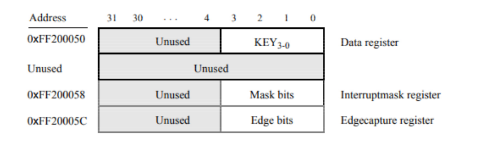Apply a mask onto the relevant memory location. E.g. to enables KEY3 and KEY0, we would:

1
2
3

LDR R1, =0xFF20058 ;; int mask addr
MOV R2, #0b1001 ;; we want to enable KEY3 and KEY0
STR R2, [R1] ;; write mask onto enable bits

When polling just grab the items at the base address. When using interrupts LDR the edge capture register to find the ones that have been pressed

Using LEDR

To display using LEDR we just need to write the value we want to the appropriate memory location. Here, assuming that what we want to display is stored in R1:

1
2

LDR R2, =0xFF2000000 ;; LEDR addr
STR [R1], R2 ;; write to LEDR

MAT292

AER210

PHY293

ESC203

n/a